Perceptron math - part 1

⸻

ANCIENT FUNDAMENTALS!

The perceptron was introduced by Frank Rosenblatt in 1957 at the Cornell Aeronautical Laboratory, inspired by early neuroscience ideas.

BINARY CLASSIFIER

Perceptrons apply a ‘sign’ function, forcing the output to be +1 or -1 (a discrete pred), which places the point being computed in one of two classes. The limitation of the perceptron is modelling linear shapes only. Note that logistic regression uses a similar formula - where $\sigma$ is the sigmoid in place of ‘sign’. LR output is a probability and therfore optimisable with gradient descent.

PERCEPTRONS FEATURES

Perceptrons are potentially the cleanest entry point for understanding how models work. They expose the core geometry:

• linear separators: any function that divides a dataset into two classes (2d,3d or hyperplane)
• hyperplanes: geometric object that generalises a line or plane to any number of dimensions - the perceptron makes decisions by slicing space with a hyperplane.
• constraints: constraints define a feasible region for w and b, on the correct side of the hyperplane
• optimisation: a greedy algorithm that pushes the hyperplane toward a configuration that satisfies all constraints - not smoothing a loss function

⸻

PERCEPTRON COMPUTATION

The function looks like this - the perceptron is a hyperplane:

$\hat{y} = \text{sign}(w \cdot x + b)$

Where:

• $x$ is the input
• $w$ is the weight vector
• $b$ is a bias
• The sign function outputs +1 or -1

EXAMPLE WALKTHROUGH

Let the input vector be:

$x = (2,\; -1)$

Let the weight vector be:

$w = (0.5,\; 1.0)$

Let the bias be:

$b = -0.2$

Now compute the score:

$w \cdot x + b$ $= (0.5)(2) + (1.0)(-1) - 0.2$ $= 1 - 1 - 0.2$ $= -0.2$

Now apply the sign function:

$\hat{y} = \text{sign}(-0.2) = -1$

The perceptron classifies this point as belonging to class –1.

⸻

VISUALISATIONS

Learning a theory is often about having a clear abstraction or sense of the topic clear in your thinking. For many a viusalisation helps. This small website was very helpful for me - https://vinizinho.net/projects/perceptron-viz/. This dynamic visualisation really makes the math crystal clear, demonstrating the learning process and the initial setup.

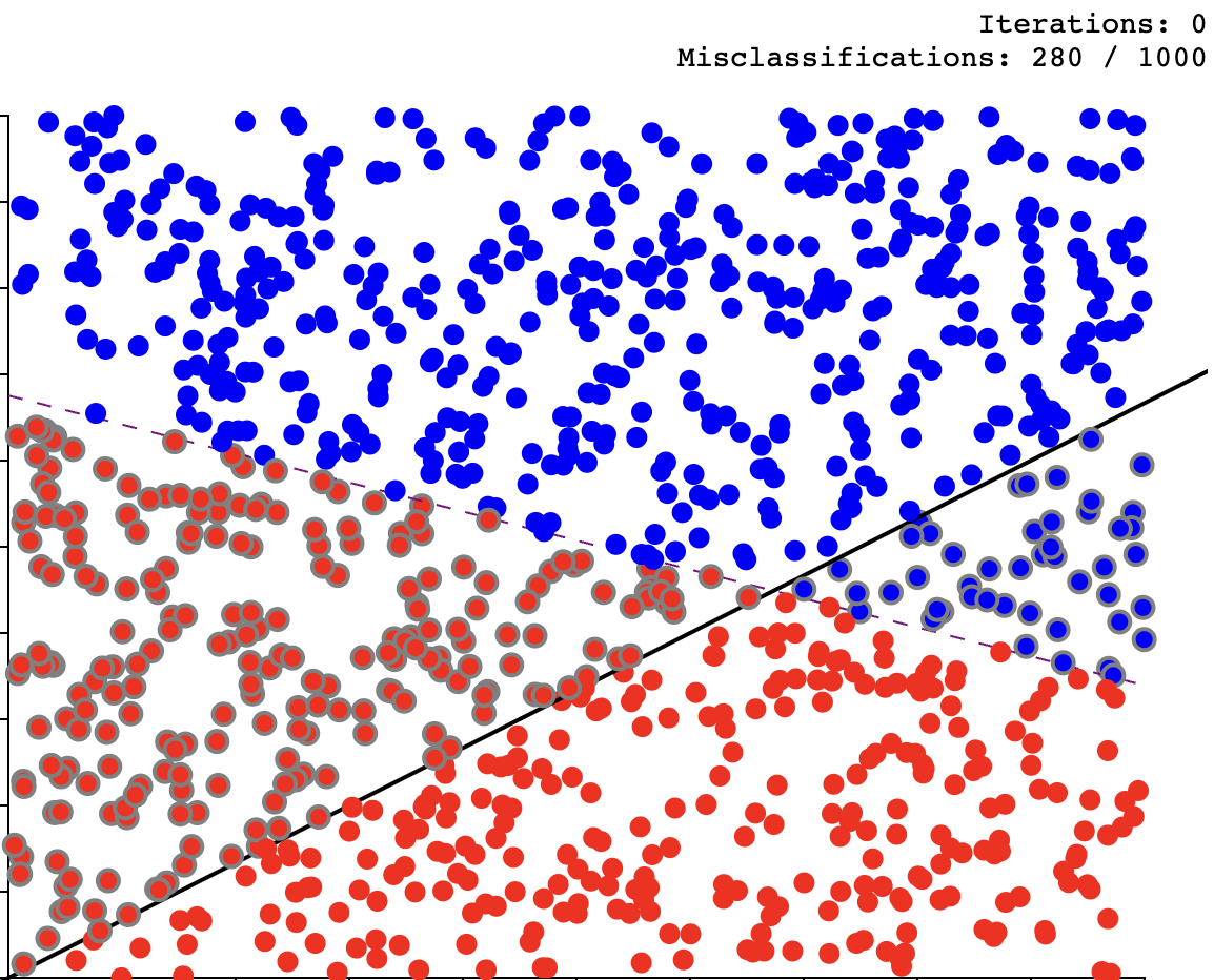
We see the two categories, the dotted ‘answer’ or correct plane and the solid line representing the initial state. Once trained fully, the solid line overlays the dotted (or is close to), each iteration causing the line to move, closer to its ultimate destination.